Our paper entitled “High-Speed, Cortex-Wide Volumetric Recording of Neuroactivity at Cellular Resolution using Light Beads Microscopy” has been published in Nature Methods.
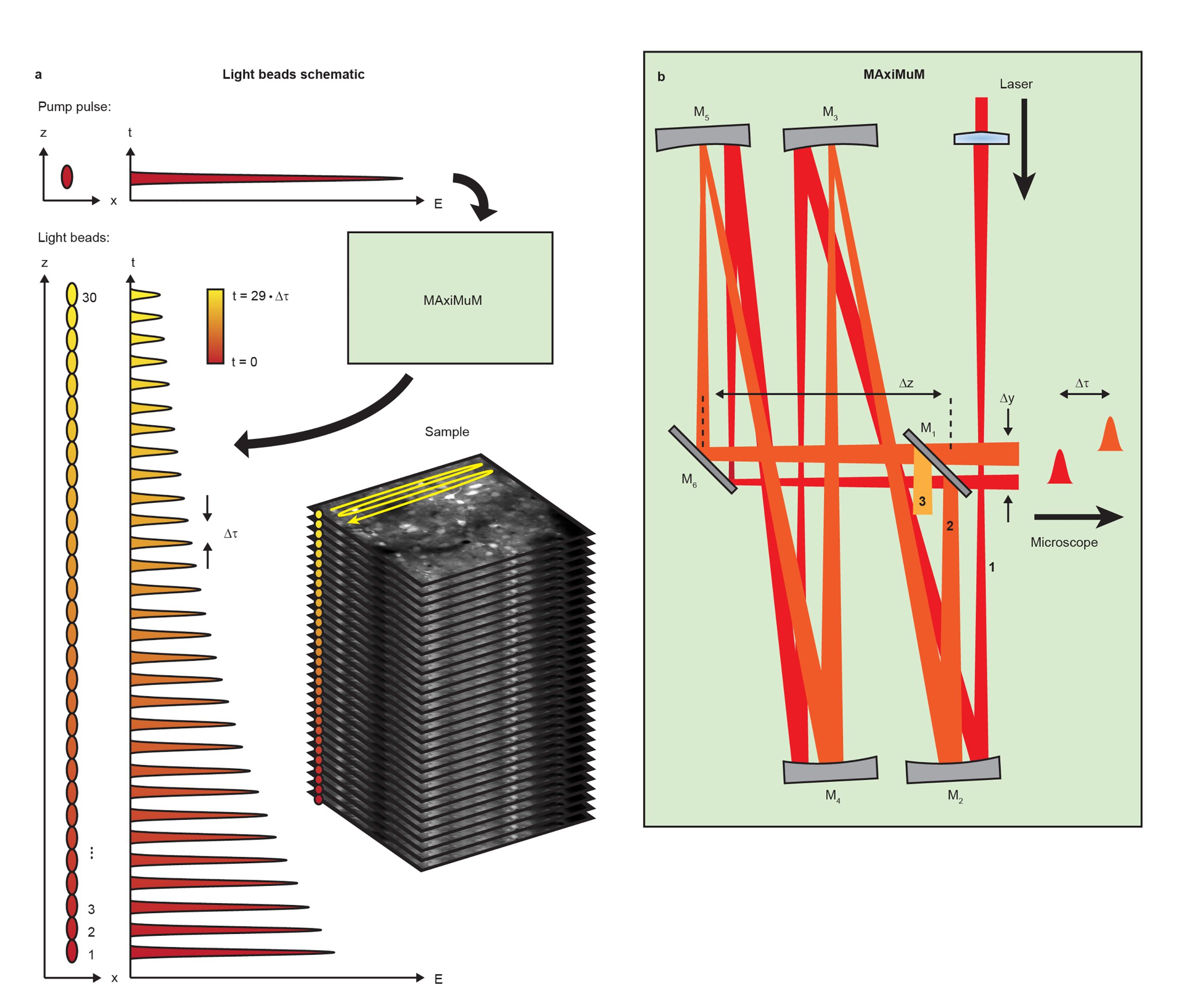
This work details our new method Light Beads Microscopy (LBM) which makes use of a column of “Light Beads” – individual beams which are distinguishable in time and focus to different depths in the sample (Fig. 1a) – in order to record from the entire depth range of a given volume within the dead time between consecutive pulses from our excitation laser. By combining LBM with a commercial mesoscope, we can image mesoscale and volumetric fields of view (FOVs) at the same rate that a conventional mesoscope records a single plane. As a result, LBM gives optical access to the activity of cortex-wide volumes, allowing recording of up to 1,000,000 neurons at calcium-imaging-compatible volume rates.
We generate our light beads using a stand-alone system called the Many-fold Axial Multiplexing Module (MAxiMuM). MAxiMuM uses a re-imaging cavity based on 4 concave mirrors (Fig. 1b). Each round trip around the cavity adds a delay, making each light bead distinguishable in time, and an axial offset in the focus of the beam. A partially reflective mirror allows beads to escape the cavity. The earliest beads have higher pulse energy and are thus directed to the deepest layers of the volume in order to combat signal reduction due to tissue scattering. By carefully tuning the transmission of the mirror, we can match the scattering profile along the axis, leading to equal signal to noise ratio for all light beads. MAxiMuM is a marked departure from previous multiplexing techniques as it allows for control of the axial separation between foci, the relative power between foci, and the total number of multiplexed beams -30-fold in this case -, roughly an order of magnitude higher than any other previous temporal multiplexing approach demonstrated in vivo.
Using LBM, we demonstrate mesoscale and volumetric recording of calcium activity in of awake and behaving mice transgenically expressing GCaMP6s in multiple regions of the cortex. We record from ~200,000 neurons within a 3 x 5 x 0.5 mm volume at 4.7 Hz comprising visual, somatosensory, posterior-parietal, and retro-splenial regions of the cortex.
Using LBM can have further shown recording from ~1,000,000 neurons within a 5.4 x 6 x 0.5 mm volume spanning both hemispheres of the mouse cortex at 2.2 Hz.
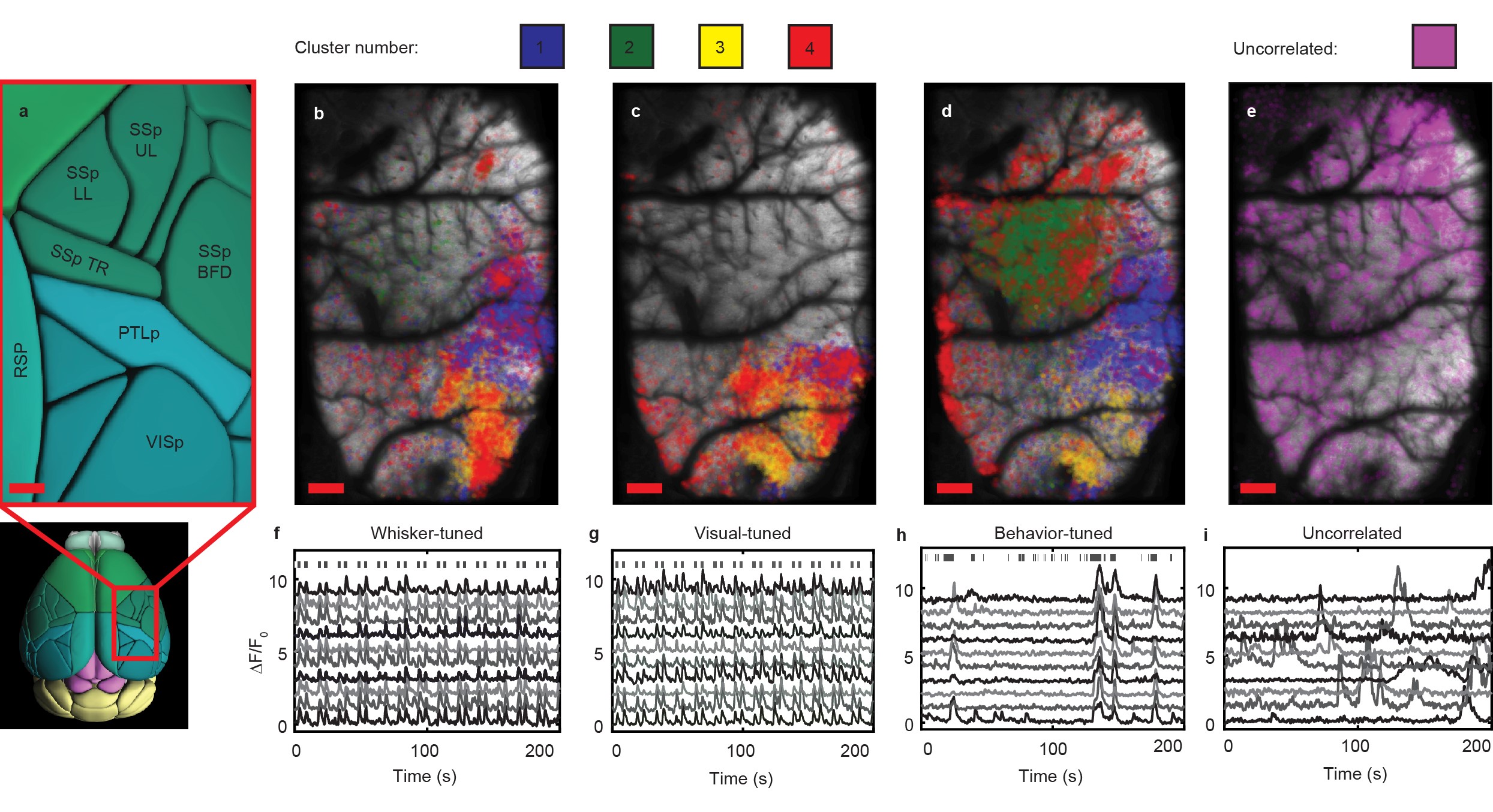
Additionally, LBM can be used to probe the spatial and temporal distributions on correlated neurons throughout multiple regions of the cortex. We considered all neurons correlated to stimulation of a mouse’s whiskers, correlated with the appearance of drifting grating visual stimuli, or correlated to spontaneous behaviors (i.e. grooming behaviors, running behaviors, or any other motion of the animal’s paws) and performed hierarchical clustering on this combined population of stimulus-tuned neurons. We mapped the neurons back to their anatomical locations within the brain (Fig. 2a), sorted by cluster and preferred stimulus (Fig. 2b-2d), and compared them to the spatial distribution of non-stimulus-correlated neurons (Fig. 2e). We find that some clusters are present in multiple stimulus conditions, suggesting some mixed selectivity of those neuronal populations. For all cases, we are able to faithfully extract the transients of single neurons within the population (Figs. 2f-2i).
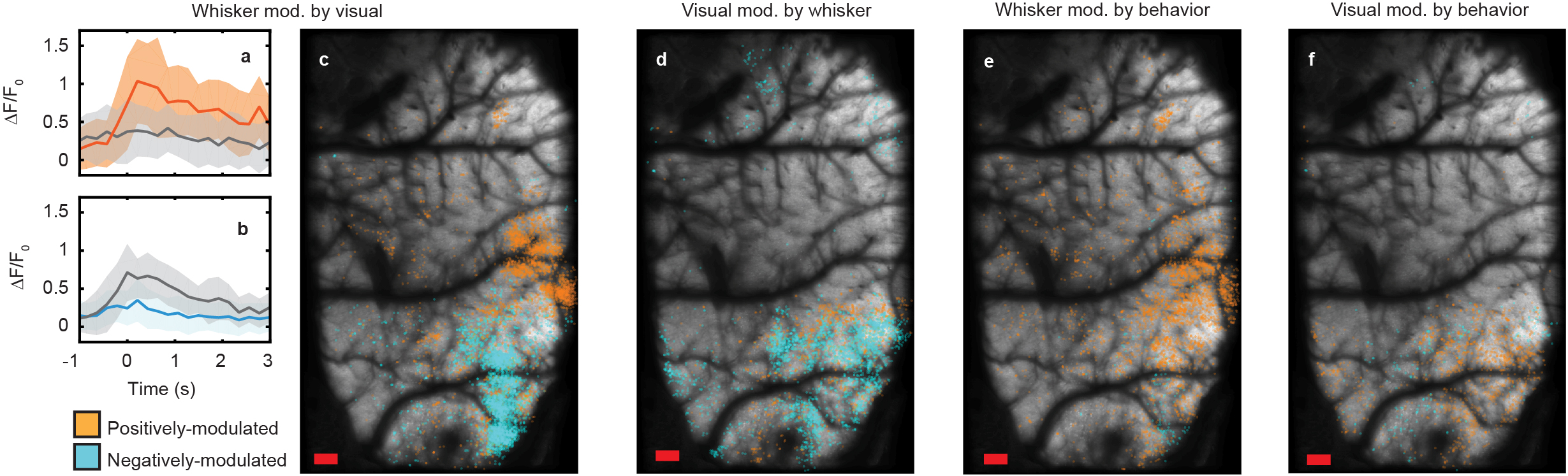
To probe mixed selectivity further, we analyzed neurons whose response is modulated by the presence of an additional stimuli. For example, Fig 3a shows the trial-averaged response of a whisker-stimulus-tuned neuron whose activity is positively modulated in the presence of coincident visual stimuli, and vice versa for Fig. 3b. Mapping the spatial locations of these neurons whose response is modulated by coincident stimuli back into anatomical space, we find that whisker-stimulus-tuned neurons can be both positively- and negatively-modulated by coincident stimuli, with a clear anatomical division between these sub-populations seeming to correspond to the division between the barrel cortex and visual cortex (Fig. 3c). In contrast, visual-tuned neurons are almost entirely negatively-modulated by the presence of whisker stimuli (Fig. 3d), and both whisker- and visual-stimulus-tuned neurons are positively-modulated by spontaneous behaviors of the animal (Figs. 3e, 3f).
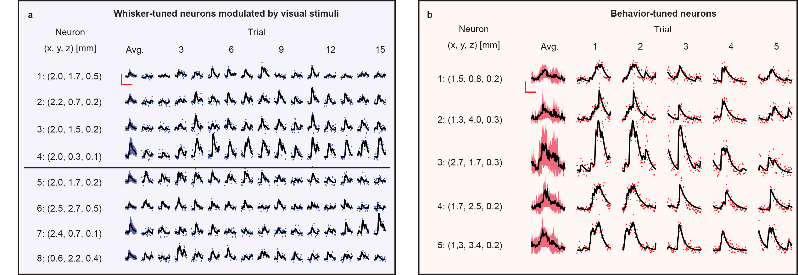
At the single trial level, we find that stimulus-tuned neurons (whisker-stimulus-tuned in Fig. 4a and behavior-tuned in Fig. 4b) vary in magnitude of response and onset time of response from trial-to-trial. Analyzing further, we found pairs of neurons whose variations in response at the single trial level co-vary significantly (r < 3σ) despite some of these neurons inhabiting different brain regions and different cortical layers. Capturing single trial dynamics on these scales underscores the need for simultaneous mesoscale and volumetric imaging technologies like LBM.
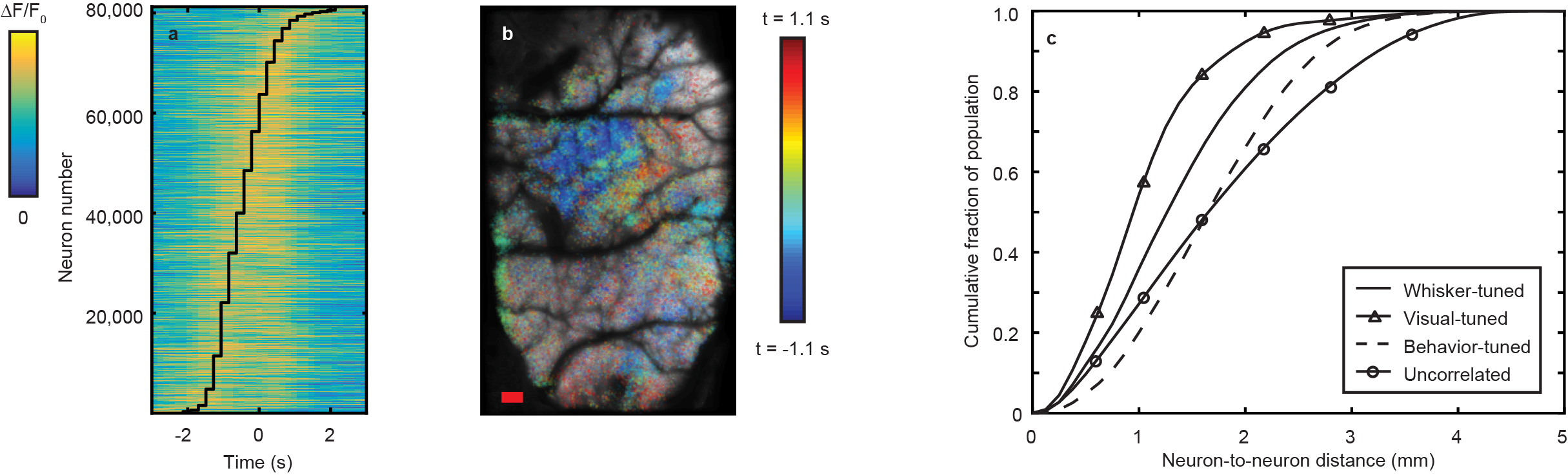
To this same point, we analyzed the variation in the onset time of neurons correlated with spontaneous behaviors of the mouse (Fig. 5a, 5b) finding that the relative lag in response between different regions of the cortex can vary on the order of seconds. Furthermore, we analyzed the pair-wise separations between pairs of neurons tuned to a given stimulus with significant (r > 3σ) correlation in their activity (Fig. 5c), finding that such pairs can span distances of 2 – 4 mm. Observing correlations on these time- and distance- scales is not possible without the increased information throughput afforded by LBM.
The above results showcase the capabilities of LBM and the range of biological questions that can be studied with it. LBM and MAxiMuM represent a modular approach to increasing the information throughput of mesoscopic imaging systems. The two-order of magnitude increase in the number of neurons accessible via LBM dramatically changes the nature of the queries regarding inter-regional, inter-layer, and dual-hemispheric neuronal networks that investigators can explore at the single-trial level.
Relevant publication:
Jeffrey Demas, Jason Manley, Frank Tejera, Kevin Barber, Hyewon Kim, Francisca Martínez Traub, Brandon Chen, and Alipasha Vaziri, High-Speed, Cortex-Wide Volumetric Recording of Neuroactivity at Cellular Resolution using Light Beads Microscopy, Nature Methods 18, pages 1103–1111 (2021); doi 10.1038/s41592-021-01239-8.
(Download)